Software installation using conda

Overview

Teaching: 15 min
Exercises: 15 min

Questions

• How do I install and manage all the Python libraries that I want to use?

• How do I interact with Python?

Objectives

• Explain the advantages of Anaconda over other Python distributions.

• Extend the number of packages available via conda using conda-forge.

• Create a conda environment with the libraries needed for these lessons.

Methods for installing packages

The setup instructions for Python for Ecologists state that we need to install the package called plotnine.

Now that we’ve identified a Python library we want to use, how do we go about installing it?

Our first impulse might be to use the Python package installer (pip), but until recently pip only worked for libraries written in pure Python. This was a major limitation for the data science community, because many scientific Python libraries have C and/or Fortran dependencies. To spare people the pain of installing these dependencies, a number of scientific Python “distributions” have been released over the years. These come with the most popular data science libraries and their dependencies pre-installed, and some also come with a package manager to assist with installing additional libraries that weren’t pre-installed. This tutorial focuses on conda, which is the package manager associated with the very popular Anaconda distribution.

Introducing conda

According to the latest documentation, Anaconda comes with over 250 of the most widely used data science libraries (and their dependencies) pre-installed. In addition, there are several thousand libraries available via the conda install command, which can be executed using the Bash Shell or Anaconda Prompt (Windows only). Linux and Mac users can open a Terminal window and execute the bash commands that way. 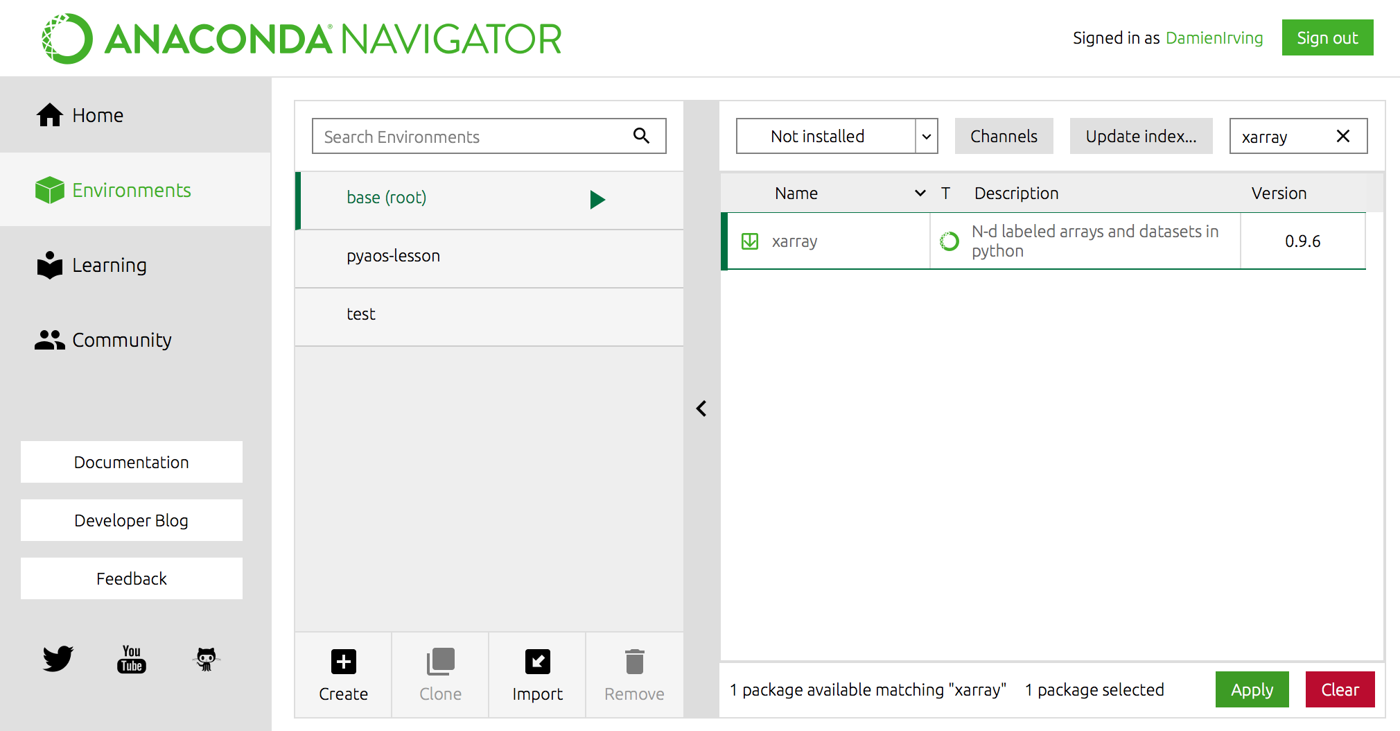It is also possible to install packages using the Anaconda Navigator graphical user interface in the “Environments” section an searching for the packages you want to install.

conda in the shell on windows

If you’re on a Windows machine and the conda command isn’t available at the Bash Shell, you’ll need to open the Anaconda Prompt program (via the Windows start menu) and run the command conda init bash (this only needs to be done once). After that, your Bash Shell will be configured to use conda going forward.

For instance, the popular xarray library could be installed using the following command,

$ conda install xarray

(Use conda search -f {package_name} to find out if a package you want is available.)

OR using Anaconda Navigator:

Miniconda

If you don’t want to install the entire Anaconda distribution, you can install Miniconda instead. It essentially comes with conda and nothing else.

Live demo

Let’s try installing our required package plotnine together. Open up an Anaconda Prompt (or Terminal if on Mac) and follow along.

Note that whenever lessons have a “Bash” section like the one shown below it means use an Anaconda Prompt (windows) or Terminal (Mac or Linux).

$ conda install -y -c conda-forge plotnine

Advanced conda

For a relatively small/niche field of research like atmosphere and ocean science, one of the most important features that Anaconda provides is the Anaconda Cloud website, where the community can contribute conda installation packages. This is critical because many of our libraries have a small user base, which means they’ll never make it into the top few thousand data science libraries supported by Anaconda.

You can search Anaconda Cloud to find the command needed to install the package. For instance, here is the search result for the iris package:

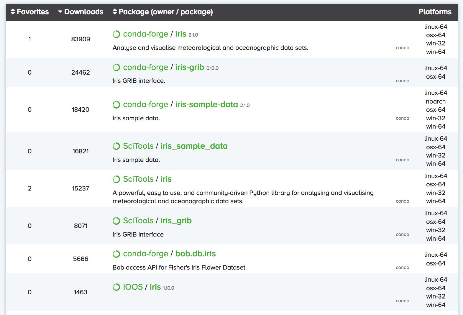
As you can see, there are often multiple versions of the same package up on Anaconda Cloud. To try and address this duplication problem, conda-forge has been launched, which aims to be a central repository that contains just a single (working) version of each package on Anaconda Cloud. You can therefore expand the selection of packages available via conda install beyond the chosen few thousand by adding the conda-forge channel:

$ conda config --add channels conda-forge

OR

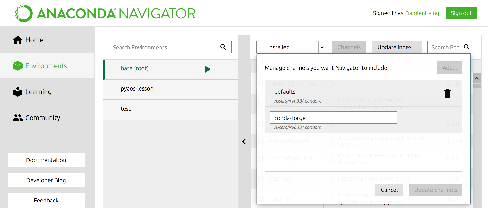
We recommend not adding any other third-party channels unless absolutely necessary, because mixing packages from multiple channels can cause headaches like binary incompatibilities.

Software installation for the lessons

xarray netCDF4 (xarray requires this to read netCDF files), cartopy (to help with geographic plot projections), cmocean (for nice color palettes), cmdline_provenance (to keep track of our data processing steps) and jupyter (so we can use the jupyter notebook).
plotnine

We could install these libraries from Anaconda Navigator (not shown) or using the Terminal in Mac/Linux or Anaconda Prompt (Windows):

$ conda install jupyter xarray netCDF4 cartopy

$ conda install -c conda-forge cmocean cmdline_provenance plotnine

If we then list all the libraries that we’ve got installed, we can see that jupyter, xarray, netCDF4, cartopy, cmocean, cmdline_provenance, plotnine and their dependencies are now there:

$ conda list

(This list can also be viewed in the environments tab of the Navigator.)

Creating separate environments

If you’ve got multiple data science projects on the go, installing all your packages in the same conda environment can get a little messy. (By default they are installed in the root/base environment.) It’s therefore common practice to create separate conda environments for the various projects you’re working on.

For instance, we could create an environment called pyaos-lesson for this lesson. The process of creating a new environment can be managed in the environments tab of the Anaconda Navigator or via the following Bash Shell / Anaconda Prompt commands:

$ conda create -n pyaos-lesson jupyter xarray netCDF4 cartopy cmocean cmdline_provenance
$ conda activate pyaos-lesson

(it’s conda deactivate to exit)

You can have lots of different environments,

$ conda info --envs

# conda environments:
#
base                  *  /anaconda3
pyaos-lesson             /anaconda3/envs/pyaos-lesson
test                     /anaconda3/envs/test

the details of which can be exported to a YAML configuration file:

$ conda env export -n pyaos-lesson -f pyaos-lesson.yml
$ cat pyaos-lesson.yml

name: pyaos-lesson
channels:
  - conda-forge
  - defaults
dependencies:
  - cartopy=0.16.0=py36h81b52dc_1
  - certifi=2018.4.16=py36_0
  - cftime=1.0.1=py36h7eb728f_0
  - ...

Other people (or you on a different computer) can then re-create that exact environment using the YAML file:

$ conda env create -f pyaos-lesson.yml

For ease of sharing the YAML file, it can be uploaded to your account at the Anaconda Cloud website,

$ conda env upload -f pyaos-lesson.yml

so that others can re-create the environment by simply refering to your Anaconda username:

$ conda env create damienirving/pyaos-lesson
$ conda activate pyaos-lesson

The ease with which others can recreate your environment (on any operating system) is a huge breakthough for reproducible research.

To delete the environment:

$ conda env remove -n pyaos-lesson

Interacting with Python

Now that we know which Python libraries we want to use and how to install them, we need to decide how we want to interact with Python.

The most simple way to use Python is to type code directly into the interpreter. This can be accessed from the bash shell:

$ python
Python 3.7.1 (default, Dec 14 2018, 13:28:58) 
[Clang 4.0.1 (tags/RELEASE_401/final)] :: Anaconda, Inc. on darwin
Type "help", "copyright", "credits" or "license" for more information.
>>> print("hello world")
hello world
>>> exit()
$

The >>> prompt indicates that you are now talking to the Python interpreter.

A more powerful alternative to the default Python interpreter is IPython (Interactive Python). The online documentation outlines all the special features that come with IPython, but as an example, it lets you execute bash shell commands without having to exit the IPython interpreter:

$ ipython
Python 3.7.1 (default, Dec 14 2018, 13:28:58) 
Type 'copyright', 'credits' or 'license' for more information
IPython 7.2.0 -- An enhanced Interactive Python. Type '?' for help.

In [1]: print("hello world")                                                    
hello world

In [2]: ls                                                                      
data/                              script_template.py
plot_precipitation_climatology.py

In [3]: exit                                                                    
$ 

(The IPython interpreter can also be accessed via the Anaconda Navigator by running the QtConsole.)

While entering commands to the Python or IPython interpreter line-by-line is great for quickly testing something, it’s clearly impractical for developing longer bodies of code and/or interactively exploring data. As such, Python users tend to do most of their code development and data exploration using either an Integrated Development Environment (IDE) or Jupyter Notebook:

• Two of the most common IDEs are Spyder and PyCharm (the former comes with Anaconda) and will look very familiar to anyone who has used MATLAB or R-Studio.
• Jupyter Notebooks run in your web browser and allow users to create and share documents that contain live code, equations, visualizations and narrative text.

We are going to use the Jupyter Notebook to explore our precipitation data (and the plotting functionality of xarray) in the next few lessons. A notebook can be launched from our data-carpentry directory using the Bash Shell:

$ cd ~/Desktop/data-carpentry
$ jupyter notebook &

(The & allows you to come back and use the bash shell without closing your notebook first.)

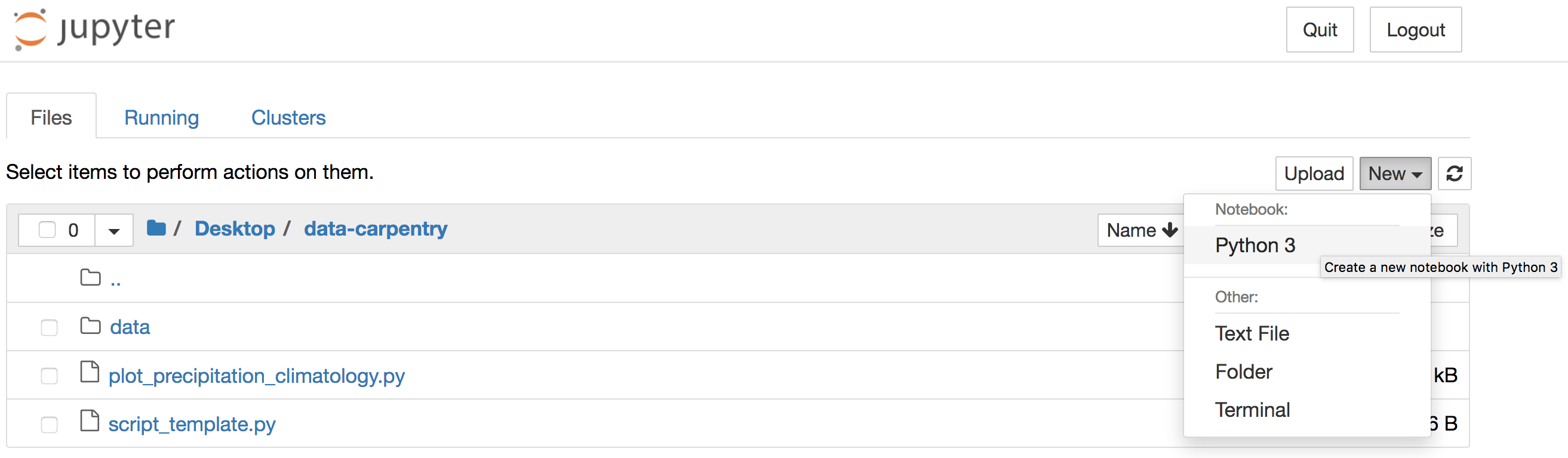
Alternatively, you can launch Jupyter Notebook from the Anaconda Navigator and navigate to the data-carpentry directory before creating a new Python 3 notebook:

JupyterLab

The Jupyter team have recently launched JupyterLab which combines the Jupyter Notebook with many of the features common to an IDE.

Install the Python libraries required for week 2

Go ahead and install jupyter, xarray, cartopy and cmocean using either the Anaconda Navigator, Bash Shell or Anaconda Prompt (Windows).

(You may like to create a separate pyaos-lesson conda environment, but this is not necessary to complete the lessons.)

Solution

The setup menu at the top of the page contains a series of drop-down boxes explaining how to install the Python libraries on different operating systems. Use the “default” instructions unless you want to create the separate pyaos-lesson conda environment.

Launch a Jupyer Notebook

In preparation for the next lesson, open a new Jupyter Notebook in your data-carpentry directory by entering jupyter notebook & at the Bash Shell or by clicking the Jupyter Notebook launch button in the Anaconda Navigator.

If you use the Navigator, the Jupyter interface will open in a new tab of your default web browser. Use that interface to navigate to the data-carpentry directory that you created specifically for these lessons before clicking to create a new Python 3 notebook:

Once your notebook is open, import xarray, catropy, matplotlib and numpy using the following Python commands:

import xarray as xr
import cartopy.crs as ccrs
import matplotlib.pyplot as plt
import numpy as np

(Hint: Hold down the shift and return keys to execute a code cell in a Jupyter Notebook.)

Key Points

• install plotnine, a required pakcage for our lessons.

• xarray and iris are the core Python libraries used in the atmosphere and ocean sciences.

• Use conda to install and manage your Python environments.